2. The Aiyagari Model#
Contents
In addition to what’s in Anaconda, this lecture will need the following libraries:
!pip install quantecon
Show code cell output
Collecting quantecon
Downloading quantecon-0.7.2-py3-none-any.whl.metadata (4.9 kB)
Requirement already satisfied: numba>=0.49.0 in /home/runner/miniconda3/envs/quantecon/lib/python3.11/site-packages (from quantecon) (0.59.0)
Requirement already satisfied: numpy>=1.17.0 in /home/runner/miniconda3/envs/quantecon/lib/python3.11/site-packages (from quantecon) (1.26.4)
Requirement already satisfied: requests in /home/runner/miniconda3/envs/quantecon/lib/python3.11/site-packages (from quantecon) (2.31.0)
Requirement already satisfied: scipy>=1.5.0 in /home/runner/miniconda3/envs/quantecon/lib/python3.11/site-packages (from quantecon) (1.11.4)
Requirement already satisfied: sympy in /home/runner/miniconda3/envs/quantecon/lib/python3.11/site-packages (from quantecon) (1.12)
Requirement already satisfied: llvmlite<0.43,>=0.42.0dev0 in /home/runner/miniconda3/envs/quantecon/lib/python3.11/site-packages (from numba>=0.49.0->quantecon) (0.42.0)
Requirement already satisfied: charset-normalizer<4,>=2 in /home/runner/miniconda3/envs/quantecon/lib/python3.11/site-packages (from requests->quantecon) (2.0.4)
Requirement already satisfied: idna<4,>=2.5 in /home/runner/miniconda3/envs/quantecon/lib/python3.11/site-packages (from requests->quantecon) (3.4)
Requirement already satisfied: urllib3<3,>=1.21.1 in /home/runner/miniconda3/envs/quantecon/lib/python3.11/site-packages (from requests->quantecon) (2.0.7)
Requirement already satisfied: certifi>=2017.4.17 in /home/runner/miniconda3/envs/quantecon/lib/python3.11/site-packages (from requests->quantecon) (2024.2.2)
Requirement already satisfied: mpmath>=0.19 in /home/runner/miniconda3/envs/quantecon/lib/python3.11/site-packages (from sympy->quantecon) (1.3.0)
Downloading quantecon-0.7.2-py3-none-any.whl (215 kB)
?25l   ━━━━━━━━━━━━━━━━━━━━━━━━━━━━━━━━━━━━━━━━ 0.0/215.4 kB ? eta -:--:--
   ━━━━━━━━━━━━━━━━━━━━━━━━━━━━━━━━━━━━━━━╸ 215.0/215.4 kB 6.9 MB/s eta 0:00:01
   ━━━━━━━━━━━━━━━━━━━━━━━━━━━━━━━━━━━━━━━━ 215.4/215.4 kB 6.3 MB/s eta 0:00:00
?25h
Installing collected packages: quantecon
Successfully installed quantecon-0.7.2
2.1. Overview#
In this lecture, we describe the structure of a class of models that build on work by Truman Bewley [Bewley, 1977].
We begin by discussing an example of a Bewley model due to Rao Aiyagari [Aiyagari, 1994].
The model features
Heterogeneous agents
A single exogenous vehicle for borrowing and lending
Limits on amounts individual agents may borrow
The Aiyagari model has been used to investigate many topics, including
precautionary savings and the effect of liquidity constraints [Aiyagari, 1994]
risk sharing and asset pricing [Heaton and Lucas, 1996]
the shape of the wealth distribution [Benhabib et al., 2015]
etc., etc., etc.
Let’s start with some imports:
import matplotlib.pyplot as plt
plt.rcParams["figure.figsize"] = (11, 5)  #set default figure size
import numpy as np
from quantecon.markov import DiscreteDP
from numba import jit
2.1.1. References#
The primary reference for this lecture is [Aiyagari, 1994].
A textbook treatment is available in chapter 18 of [Ljungqvist and Sargent, 2018].
A continuous time version of the model by SeHyoun Ahn and Benjamin Moll can be found here.
2.2. The Economy#
2.2.1. Households#
Infinitely lived households / consumers face idiosyncratic income shocks.
A unit interval of ex-ante identical households face a common borrowing constraint.
The savings problem faced by a typical household is
subject to
where
\(c_t\) is current consumption
\(a_t\) is assets
\(z_t\) is an exogenous component of labor income capturing stochastic unemployment risk, etc.
\(w\) is a wage rate
\(r\) is a net interest rate
\(B\) is the maximum amount that the agent is allowed to borrow
The exogenous process \(\{z_t\}\) follows a finite state Markov chain with given stochastic matrix \(P\).
The wage and interest rate are fixed over time.
In this simple version of the model, households supply labor inelastically because they do not value leisure.
2.3. Firms#
Firms produce output by hiring capital and labor.
Firms act competitively and face constant returns to scale.
Since returns to scale are constant the number of firms does not matter.
Hence we can consider a single (but nonetheless competitive) representative firm.
The firm’s output is
where
\(A\) and \(\alpha\) are parameters with \(A > 0\) and \(\alpha \in (0, 1)\)
\(K_t\) is aggregate capital
\(N\) is total labor supply (which is constant in this simple version of the model)
The firm’s problem is
The parameter \(\delta\) is the depreciation rate.
From the first-order condition with respect to capital, the firm’s inverse demand for capital is
Using this expression and the firm’s first-order condition for labor, we can pin down the equilibrium wage rate as a function of \(r\) as
2.3.1. Equilibrium#
We construct a stationary rational expectations equilibrium (SREE).
In such an equilibrium
prices induce behavior that generates aggregate quantities consistent with the prices
aggregate quantities and prices are constant over time
In more detail, an SREE lists a set of prices, savings and production policies such that
households want to choose the specified savings policies taking the prices as given
firms maximize profits taking the same prices as given
the resulting aggregate quantities are consistent with the prices; in particular, the demand for capital equals the supply
aggregate quantities (defined as cross-sectional averages) are constant
In practice, once parameter values are set, we can check for an SREE by the following steps
pick a proposed quantity \(K\) for aggregate capital
determine corresponding prices, with interest rate \(r\) determined by (2.1) and a wage rate \(w(r)\) as given in (2.2)
determine the common optimal savings policy of the households given these prices
compute aggregate capital as the mean of steady state capital given this savings policy
If this final quantity agrees with \(K\) then we have a SREE.
2.4. Code#
Let’s look at how we might compute such an equilibrium in practice.
To solve the household’s dynamic programming problem we’ll use the DiscreteDP class from QuantEcon.py.
Our first task is the least exciting one: write code that maps parameters for a household problem into the R and Q matrices needed to generate an instance of DiscreteDP.
Below is a piece of boilerplate code that does just this.
In reading the code, the following information will be helpful
Rneeds to be a matrix whereR[s, a]is the reward at statesunder actiona.Qneeds to be a three-dimensional array whereQ[s, a, s']is the probability of transitioning to states'when the current state issand the current action isa.
(A more detailed discussion of DiscreteDP is available in the Discrete State Dynamic Programming lecture in the Advanced
Quantitative Economics with Python lecture series.)
Here we take the state to be \(s_t := (a_t, z_t)\), where \(a_t\) is assets and \(z_t\) is the shock.
The action is the choice of next period asset level \(a_{t+1}\).
We use Numba to speed up the loops so we can update the matrices efficiently when the parameters change.
The class also includes a default set of parameters that we’ll adopt unless otherwise specified.
class Household:
    """
    This class takes the parameters that define a household asset accumulation
    problem and computes the corresponding reward and transition matrices R
    and Q required to generate an instance of DiscreteDP, and thereby solve
    for the optimal policy.

    Comments on indexing: We need to enumerate the state space S as a sequence
    S = {0, ..., n}.  To this end, (a_i, z_i) index pairs are mapped to s_i
    indices according to the rule

        s_i = a_i * z_size + z_i

    To invert this map, use

        a_i = s_i // z_size  (integer division)
        z_i = s_i % z_size

    """


    def __init__(self,
                r=0.01,                      # Interest rate
                w=1.0,                       # Wages
                β=0.96,                      # Discount factor
                a_min=1e-10,
                Π=[[0.9, 0.1], [0.1, 0.9]],  # Markov chain
                z_vals=[0.1, 1.0],           # Exogenous states
                a_max=18,
                a_size=200):

        # Store values, set up grids over a and z
        self.r, self.w, self.β = r, w, β
        self.a_min, self.a_max, self.a_size = a_min, a_max, a_size

        self.Π = np.asarray(Π)
        self.z_vals = np.asarray(z_vals)
        self.z_size = len(z_vals)

        self.a_vals = np.linspace(a_min, a_max, a_size)
        self.n = a_size * self.z_size

        # Build the array Q
        self.Q = np.zeros((self.n, a_size, self.n))
        self.build_Q()

        # Build the array R
        self.R = np.empty((self.n, a_size))
        self.build_R()

    def set_prices(self, r, w):
        """
        Use this method to reset prices. Calling the method will trigger a
        re-build of R.
        """
        self.r, self.w = r, w
        self.build_R()

    def build_Q(self):
        populate_Q(self.Q, self.a_size, self.z_size, self.Π)

    def build_R(self):
        self.R.fill(-np.inf)
        populate_R(self.R,
                self.a_size,
                self.z_size,
                self.a_vals,
                self.z_vals,
                self.r,
                self.w)


# Do the hard work using JIT-ed functions

@jit(nopython=True)
def populate_R(R, a_size, z_size, a_vals, z_vals, r, w):
    n = a_size * z_size
    for s_i in range(n):
        a_i = s_i // z_size
        z_i = s_i % z_size
        a = a_vals[a_i]
        z = z_vals[z_i]
        for new_a_i in range(a_size):
            a_new = a_vals[new_a_i]
            c = w * z + (1 + r) * a - a_new
            if c > 0:
                R[s_i, new_a_i] = np.log(c)  # Utility

@jit(nopython=True)
def populate_Q(Q, a_size, z_size, Π):
    n = a_size * z_size
    for s_i in range(n):
        z_i = s_i % z_size
        for a_i in range(a_size):
            for next_z_i in range(z_size):
                Q[s_i, a_i, a_i*z_size + next_z_i] = Π[z_i, next_z_i]


@jit(nopython=True)
def asset_marginal(s_probs, a_size, z_size):
    a_probs = np.zeros(a_size)
    for a_i in range(a_size):
        for z_i in range(z_size):
            a_probs[a_i] += s_probs[a_i*z_size + z_i]
    return a_probs
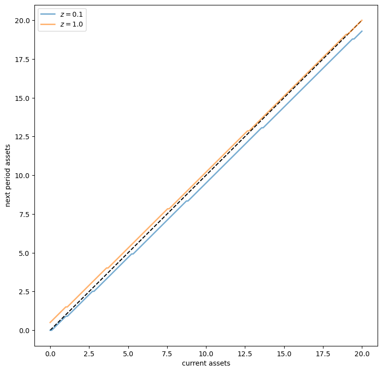
As a first example of what we can do, let’s compute and plot an optimal accumulation policy at fixed prices.
# Example prices
r = 0.03
w = 0.956

# Create an instance of Household
am = Household(a_max=20, r=r, w=w)

# Use the instance to build a discrete dynamic program
am_ddp = DiscreteDP(am.R, am.Q, am.β)

# Solve using policy function iteration
results = am_ddp.solve(method='policy_iteration')

# Simplify names
z_size, a_size = am.z_size, am.a_size
z_vals, a_vals = am.z_vals, am.a_vals
n = a_size * z_size

# Get all optimal actions across the set of a indices with z fixed in each row
a_star = np.empty((z_size, a_size))
for s_i in range(n):
    a_i = s_i // z_size
    z_i = s_i % z_size
    a_star[z_i, a_i] = a_vals[results.sigma[s_i]]

fig, ax = plt.subplots(figsize=(9, 9))
ax.plot(a_vals, a_vals, 'k--')  # 45 degrees
for i in range(z_size):
    lb = f'$z = {z_vals[i]:.2}$'
    ax.plot(a_vals, a_star[i, :], lw=2, alpha=0.6, label=lb)
    ax.set_xlabel('current assets')
    ax.set_ylabel('next period assets')
ax.legend(loc='upper left')

plt.show()

The plot shows asset accumulation policies at different values of the exogenous state.
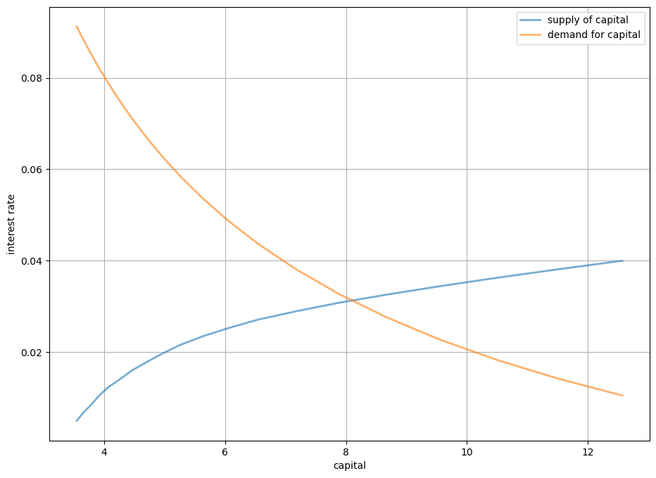
Now we want to calculate the equilibrium.
Let’s do this visually as a first pass.
The following code draws aggregate supply and demand curves.
The intersection gives equilibrium interest rates and capital.
A = 1.0
N = 1.0
α = 0.33
β = 0.96
δ = 0.05


def r_to_w(r):
    """
    Equilibrium wages associated with a given interest rate r.
    """
    return A * (1 - α) * (A * α / (r + δ))**(α / (1 - α))

def rd(K):
    """
    Inverse demand curve for capital.  The interest rate associated with a
    given demand for capital K.
    """
    return A * α * (N / K)**(1 - α) - δ


def prices_to_capital_stock(am, r):
    """
    Map prices to the induced level of capital stock.

    Parameters:
    ----------

    am : Household
        An instance of an aiyagari_household.Household
    r : float
        The interest rate
    """
    w = r_to_w(r)
    am.set_prices(r, w)
    aiyagari_ddp = DiscreteDP(am.R, am.Q, β)
    # Compute the optimal policy
    results = aiyagari_ddp.solve(method='policy_iteration')
    # Compute the stationary distribution
    stationary_probs = results.mc.stationary_distributions[0]
    # Extract the marginal distribution for assets
    asset_probs = asset_marginal(stationary_probs, am.a_size, am.z_size)
    # Return K
    return np.sum(asset_probs * am.a_vals)


# Create an instance of Household
am = Household(a_max=20)

# Use the instance to build a discrete dynamic program
am_ddp = DiscreteDP(am.R, am.Q, am.β)

# Create a grid of r values at which to compute demand and supply of capital
num_points = 20
r_vals = np.linspace(0.005, 0.04, num_points)

# Compute supply of capital
k_vals = np.empty(num_points)
for i, r in enumerate(r_vals):
    k_vals[i] = prices_to_capital_stock(am, r)

# Plot against demand for capital by firms
fig, ax = plt.subplots(figsize=(11, 8))
ax.plot(k_vals, r_vals, lw=2, alpha=0.6, label='supply of capital')
ax.plot(k_vals, rd(k_vals), lw=2, alpha=0.6, label='demand for capital')
ax.grid()
ax.set_xlabel('capital')
ax.set_ylabel('interest rate')
ax.legend(loc='upper right')

plt.show()

